在數學的數值分析領域中,貝茲曲線(英語:Bézier curve)是電腦圖學中相當重要的參數曲線。
雖然會有點排斥困難的新事物,但為了快速的解決遇到的問題,所以還是踏進貝茲曲線的世界。
其實Max在處理字型時,一直遇到貝茲曲線的問題,但一直無法有效的解決。
後來 Google 一下就找到解法,還好囫圇吞棗是Max的強項,閉著眼睛就上手了,呵呵。
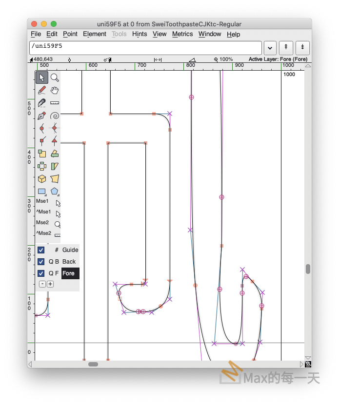
最後讓Max終於不得不去學貝茲曲線是「姵」這一個字。

Max預期要移到新的坐標是 [880,738] ,可是Max自己亂寫的code 會判斷為 [878,199] 就是上圖畫面中正間的橘點,是錯的非常離譜,但自己動腦去寫又覺得很難,感謝已經有好心人幫忙寫出實用的工具。
工具下載:
github:
https://github.com/dhermes/bezier
document:
https://bezier.readthedocs.io/en/stable/python/reference/bezier.curve.html
安裝:
The bezier Python package can be installed with pip:
$ python -m pip install --upgrade bezier
$ python3 -m pip install --upgrade bezier
$ python -m pip install --upgrade bezier[full]
解決 bezier 無法在 python3.9 安裝的問題
請服用下面解法:
BEZIER_NO_EXTENSION=true \
python3 -m pip install --upgrade bezier --no-binary=bezier
資料來源:
https://github.com/dhermes/bezier/issues/243
Why Bézier?
A Bézier curve (and triangle, etc.) is a parametric curve that uses the Bernstein basis:
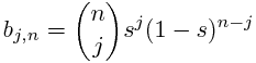
to define a curve as a linear combination:
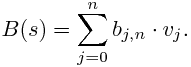
This comes from the fact that the weights sum to one:

This can be generalized to higher order by considering three, four, etc. non-negative weights that sum to one (in the above we have the two non-negative weights s and 1 - s).
Due to their simple form, Bézier curves:
- can easily model geometric objects as parametric curves, triangles, etc.
- can be computed in an efficient and numerically stable way via de Casteljau’s algorithm
- can utilize convex optimization techniques for many algorithms (such as curve-curve intersection), since curves (and triangles, etc.) are convex combinations of the basis
Many applications — as well as the history of their development — are described in “The Bernstein polynomial basis: A centennial retrospective“, for example;
- aids physical analysis using finite element methods (FEM) on isogeometric models by using geometric shape functions called NURBS to represent data
- used in robust control of dynamic systems; utilizes convexity to create a hull of curves
Getting Started
For example, to create a curve:
>>> nodes1 = np.asfortranarray([
...     [0.0, 0.5, 1.0],
...     [0.0, 1.0, 0.0],
... ])
>>> curve1 = bezier.Curve(nodes1, degree=2)
The intersection (points) between two curves can also be determined:
>>> nodes2 = np.asfortranarray([
...     [0.0, 0.25,  0.5, 0.75, 1.0],
...     [0.0, 2.0 , -2.0, 2.0 , 0.0],
... ])
>>> curve2 = bezier.Curve.from_nodes(nodes2)
>>> intersections = curve1.intersect(curve2)
>>> intersections
array([[0.31101776, 0.68898224, 0. , 1. ],
       [0.31101776, 0.68898224, 0. , 1. ]])
>>> s_vals = np.asfortranarray(intersections[0, :])
>>> points = curve1.evaluate_multi(s_vals)
>>> points
array([[0.31101776, 0.68898224, 0. , 1. ],
       [0.42857143, 0.42857143, 0. , 0. ]])
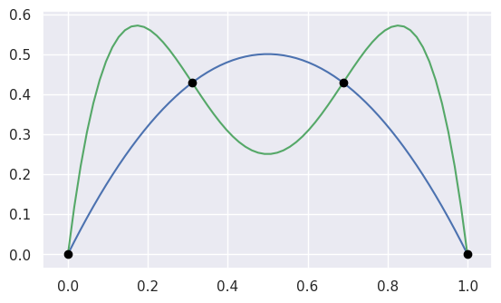
and then we can plot these curves (along with their intersections):
>>> import seaborn
>>> seaborn.set()
>>>
>>> ax = curve1.plot(num_pts=256)
>>> _ = curve2.plot(num_pts=256, ax=ax)
>>> lines = ax.plot(
...     points[0, :], points[1, :],
...     marker="o", linestyle="None", color="black")
>>> _ = ax.axis("scaled")
>>> _ = ax.set_xlim(-0.125, 1.125)
>>> _ = ax.set_ylim(-0.0625, 0.625)
For API-level documentation, check out the Bézier Python package documentation.
Development
To work on adding a feature or to run the functional tests, see the DEVELOPMENT doc for more information on how to get started.
Citation
For publications that use bezier, there is a JOSS paper that can be cited. The following BibTeX entry can be used:
@article{Hermes2017,
  doi = {10.21105/joss.00267},
  url = {https://doi.org/10.21105%2Fjoss.00267},
  year = {2017},
  month = {Aug},
  publisher = {The Open Journal},
  volume = {2},
  number = {16},
  pages = {267},
  author = {Danny Hermes},
  title = {Helper for B{\'{e}}zier Curves, Triangles, and Higher Order Objects},
  journal = {The Journal of Open Source Software}
}
A particular version of this library can be cited via a Zenodo DOI; see a full list by version.
Max 只用到2個函數分別是 evaluate() 和 locate().
evaluate(s)
Evaluate 𝐵(𝑠)B(s) along the curve.
This method acts as a (partial) inverse to locate().
See evaluate_multi() for more details.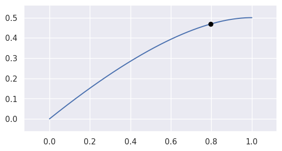
>>> nodes = np.asfortranarray([
...     [0.0, 0.625, 1.0],
...     [0.0, 0.5  , 0.5],
... ])
>>> curve = bezier.Curve(nodes, degree=2)
>>> curve.evaluate(0.75)
array([[0.796875],
       [0.46875 ]])
Parameters
s (float) – Parameter along the curve.Returns
The point on the curve (as a two dimensional NumPy array with a single column).Return type
locate(point)
Find a point on the current curve.
Solves for 𝑠s in 𝐵(𝑠)=𝑝B(s)=p.
This method acts as a (partial) inverse to evaluate().
Note
A unique solution is only guaranteed if the current curve has no self-intersections. This code assumes, but doesn’t check, that this is true.
>>> nodes = np.asfortranarray([
...     [0.0, -1.0, 1.0, -0.75 ],
...     [2.0,  0.0, 1.0,  1.625],
... ])
>>> curve = bezier.Curve(nodes, degree=3)
>>> point1 = np.asfortranarray([
...     [-0.09375 ],
...     [ 0.828125],
... ])
>>> curve.locate(point1)
0.5
>>> point2 = np.asfortranarray([
...     [0.0],
...     [1.5],
... ])
>>> curve.locate(point2) is None
True
>>> point3 = np.asfortranarray([
...     [-0.25 ],
...     [ 1.375],
... ])
>>> curve.locate(point3) is None
Traceback (most recent call last):
  ...
ValueError: Parameters not close enough to one another
Parameters
point (numpy.ndarray) – A (D x 1) point on the curve, where 𝐷D is the dimension of the curve.Returns
The parameter value (𝑠s) corresponding to point or None if the point is not on the curve.Return type
ValueError – If the dimension of the point doesn’t match the dimension of the current curve.
主要是先使用 get_distance 取得長度後,再使用 evaluate () 就可以取得該長度下的坐標位置。範例程式:
distance = spline_util.get_distance(point1[0],point1[1],point2[0],point2[1])
round_offset = 33
round_offset_rate = round_offset / distance
print('distance:',distance)
print('round_offset:',round_offset)
print('round_offset_rate:',round_offset_rate)
print(curve.evaluate(round_offset_rate))